Essential Guide To Generating And Manipulating Matrices In Matlab For Beginners

Matrices are the backbone of numerical computing in MATLAB. Whether you're analyzing data, solving systems of equations, or simulating dynamic models, a solid grasp of matrix handling is essential. For beginners, understanding how to generate, modify, and operate on matrices unlocks the full potential of MATLAB’s computational environment. This guide walks through foundational techniques with clear examples, practical tips, and real-world context to help you build confidence quickly.

Understanding Matrices in MATLAB

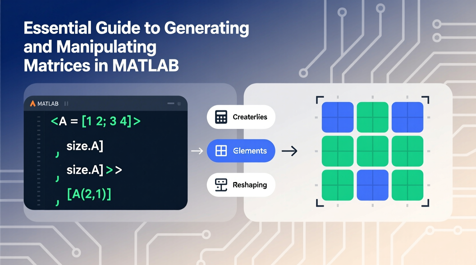
In MATLAB, all variables are treated as arrays, and matrices are two-dimensional arrays used to store numbers in rows and columns. Unlike traditional programming languages that require explicit loops for array operations, MATLAB supports vectorized computation—meaning entire matrices can be manipulated with single commands. This design makes it exceptionally efficient for mathematical and engineering tasks.

A matrix in MATLAB is defined using square brackets []. Elements in a row are separated by spaces or commas, and rows are separated by semicolons. For example:

A = [1 2 3; 4 5 6; 7 8 9];

This creates a 3×3 matrix where the first row contains 1, 2, 3, the second row has 4, 5, 6, and so on. You can view the result simply by typing the variable name in the command window.

Tip: Use the whos command to inspect the size, class, and memory usage of any matrix variable.

Creating Common Types of Matrices

While manually entering values works for small datasets, MATLAB provides built-in functions to generate standard matrices efficiently. These are especially useful when initializing large arrays or testing algorithms.

Matrix Type	MATLAB Command	Description
Zeros Matrix	zeros(3)	Creates a 3×3 matrix filled with zeros.
Ones Matrix	ones(2,4)	Generates a 2×4 matrix with all elements equal to 1.
Identity Matrix	eye(4)	Returns a 4×4 identity matrix (1s on diagonal, 0s elsewhere).
Random Matrix	rand(3,2)	Produces a 3×2 matrix with uniformly distributed random numbers between 0 and 1.
Linearly Spaced Vector	linspace(0,10,5)	Creates a row vector with 5 equally spaced points from 0 to 10.

These functions eliminate repetitive coding and reduce errors during setup. For instance, if you’re modeling temperature distribution across a grid, starting with a zeros(100,100) matrix allows you to populate only the relevant cells later.

Basic Matrix Operations and Manipulations

Once a matrix is created, you’ll often need to modify its structure or perform arithmetic. MATLAB supports intuitive syntax for both element-wise and algebraic operations.

Arithmetic Operations

• Addition/Subtraction: C = A + B adds corresponding elements of matrices A and B (must be same size).
• Matrix Multiplication: C = A * B performs standard linear algebra multiplication (inner dimensions must match).
• Element-wise Multiplication: C = A .* B multiplies each element individually (use dot operator).
• Transposition: B = A' flips rows and columns—essential for vector operations.

Indexing and Subsetting

You can access specific elements using parentheses. The syntax is A(row, column). For example:

value = A(2,3);  % Gets element in 2nd row, 3rd column
row2 = A(2,:);   % Extracts entire second row
col1 = A(:,1);   % Extracts entire first column

To replace values:

A(1,1) = 10;     % Sets top-left element to 10

“Mastering indexing early on dramatically improves your ability to debug and optimize MATLAB code.” — Dr. Linda Chen, Computational Scientist at MIT

Step-by-Step: Building and Transforming a Data Matrix

Consider a scenario where you collect sensor readings over time. Each row represents a time step, and each column records a different sensor output. Here's how to build and process such a dataset.

1. Create initial data: Simulate 5 time steps with 3 sensors.

data = rand(5,3);

2. Add timestamps: Prepend a time column starting at 0 seconds, increasing by 0.5-second intervals.

time = (0:0.5:2)';           % Column vector of times
  data_with_time = [time, data]; % Concatenate horizontally

3. Normalize sensor values: Scale each sensor’s data to range between 0 and 1.

scaled_data = data_with_time;
  for i = 2:4
      col = scaled_data(:,i);
      scaled_data(:,i) = (col - min(col)) / (max(col) - min(col));
  end

4. Extract high-readings: Find all entries above 0.8.

high_values = scaled_data(scaled_data(:,2:4) > 0.8);

This sequence demonstrates how matrices evolve from raw input to processed insight using basic MATLAB tools. No external libraries are needed—everything relies on core functionality.

Tip: Use logical indexing (like A(A > 5)) to extract or modify elements based on conditions—this avoids loops and speeds up execution.

Common Pitfalls and Best Practices Checklist

New users often encounter avoidable errors due to misunderstanding syntax or dimension rules. The following checklist helps prevent common issues:

• ✅ Always ensure matrix dimensions match before addition or multiplication.
• ✅ Use .*, ./, and .^ for element-wise operations—not *, /, ^.
• ✅ Prefer vectorized operations over loops whenever possible for better performance.
• ✅ Clear variables with clear or use clc to clean the command window during testing.
• ✅ Name matrices descriptively (e.g., temperatureData instead of T) for readability.
• ✅ Use comments (%) to explain complex lines, especially in longer scripts.

Avoid mixing scalars, vectors, and matrices without verifying compatibility. For example, multiplying a 3×3 matrix by a 1×3 vector will fail unless transposed correctly.

Frequently Asked Questions

How do I create a diagonal matrix from a vector?

Use the diag() function. If v = [1 2 3], then D = diag(v) creates a 3×3 matrix with 1, 2, 3 on the main diagonal and zeros elsewhere.

Can I concatenate matrices vertically and horizontally?

Yes. Use [A; B] to stack matrices vertically (requires same number of columns), and [A, B] to place them side by side (same number of rows). Mismatched sizes will trigger an error.

What does the colon operator do in indexing?

The colon : means \"all elements\" in a dimension. So A(:,2) selects all rows in column 2, while A(3,:) grabs all columns in row 3. It’s one of MATLAB’s most powerful features for slicing data.

Conclusion: Start Applying Matrix Skills Today

Generating and manipulating matrices in MATLAB is not just a technical skill—it's the foundation for exploring data, building simulations, and solving real engineering problems. From creating simple arrays to performing advanced transformations, every operation builds toward greater fluency in scientific computing. With consistent practice, these tools become second nature.

🚀 Ready to level up? Open MATLAB now, try creating a 4×4 magic square with magic(4), and experiment with transposing, summing rows, or extracting submatrices. Share your results or questions in the community forums to deepen your learning!