Mastering Drop Down Box Editing In Excel A Step By Step Guide For Custom Lists

Drop down boxes in Excel—also known as data validation lists—are powerful tools that bring structure, consistency, and professionalism to your spreadsheets. Whether you're managing inventory, tracking project statuses, or organizing employee schedules, a well-designed drop down list reduces errors, speeds up data entry, and enhances user experience. While many users know how to insert a basic list, true mastery lies in creating dynamic, reusable, and intelligent custom lists tailored to your workflow. This guide walks through the full process—from setup to advanced customization—with practical tips and real-world applications.

Why Custom Drop Down Lists Matter

Standard data entry is prone to typos, inconsistent formatting, and invalid inputs. For example, one person might type “In Progress,” while another enters “in progress” or “IP.” These variations make filtering, sorting, and analyzing data difficult. A custom drop down list eliminates such inconsistencies by offering predefined options.

Beyond error prevention, custom lists improve collaboration. Team members don’t need to guess acceptable values—they simply select from a controlled menu. This is especially useful in shared workbooks where multiple users input data across departments or time zones.

“Structured data entry isn’t just about neatness—it’s about data integrity. A single typo can derail an entire report.” — David Lin, Data Analyst & Excel Trainer

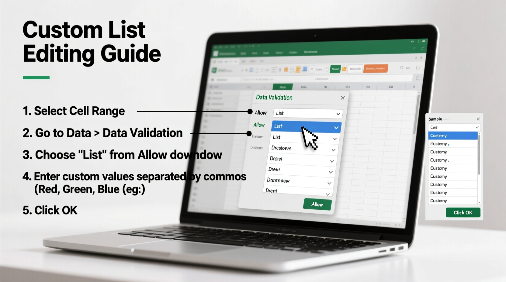
Step-by-Step: Creating Your First Custom Drop Down List

Follow this sequence to build a functional drop down box using a custom list:

1. Prepare Your Source List: Type your desired options into a single column or row (e.g., A1:A5). For instance:
   • A1: Not Started
   • A2: In Progress
   • A3: On Hold
   • A4: Completed
   • A5: Cancelled
2. Select Target Cells: Highlight the cells where you want the drop down (e.g., D2:D100).
3. Open Data Validation: Go to the Data tab → Click Data Validation.
4. Set Validation Criteria: In the dialog box, under Allow, choose “List.”
5. Enter Source Range: In the Source field, enter the reference to your list (e.g., =$A$1:$A$5).
6. Confirm and Test: Click OK. Click any target cell—you should now see a drop down arrow with your options.

Tip: Always use absolute references (with $ signs) when defining your source range to prevent errors when copying formulas or applying validation to multiple cells.

Enhancing Usability with Named Ranges

Hardcoding cell ranges like $A$1:$A$5 works for simple cases, but it becomes problematic when inserting or deleting rows. A better approach is to use named ranges.

To create one:

1. Select your list (e.g., A1:A5).
2. Go to the Formulas tab → Click Define Name.
3. Name it something meaningful like “ProjectStatusOptions”.
4. In the Data Validation dialog, use =ProjectStatusOptions as the source.

Now, if you insert a new status between rows, the named range automatically expands (if using Excel Tables) or can be manually adjusted without changing every validation rule.

Advanced Technique: Dynamic Drop Downs Using Tables

To future-proof your lists, convert your source data into an Excel Table (Ctrl + T). Tables automatically expand when you add new entries, making them ideal for evolving lists.

After converting your list to a Table:

1. Name the column containing your options (e.g., “StatusList[Status]”).
2. In Data Validation, set Source to =INDIRECT(\"StatusList[Status]\") or directly reference the structured table column.

This ensures that whenever someone adds a new option to the table, it instantly appears in all associated drop downs—no manual updates required.

Common Pitfalls and How to Avoid Them

Even experienced users make mistakes when working with drop down boxes. Here are frequent issues and their solutions:

Issue	Solution
Drop down doesn't update after adding new items	Use a Table with a named range instead of static cell references.
User can still type invalid values	Ensure “Ignore blank” is unchecked and consider enabling “Show error alert after invalid data is entered.”
List source moves or breaks	Avoid relative references; always anchor ranges or use names.
Drop down arrows not visible	Check zoom level—arrows disappear below 30%. Also ensure no merged cells interfere.

Real-World Example: Project Tracker Implementation

Consider a marketing team managing 20 campaigns across four regions. They use Excel to track each campaign’s status. Initially, team members typed statuses freely, leading to over 12 variations of “Pending” and “Done.” Reports were unreliable.

After implementing a custom drop down using a named range called “CampaignStatus,” all users selected from standardized options: Draft, Active, Paused, Completed, Cancelled. The change reduced data cleanup time by 70% and improved dashboard accuracy overnight.

Additionally, they linked the list to a Table so managers could add new statuses (like “Under Review”) without disrupting existing sheets. The system scaled seamlessly as processes evolved.

Pro Tips for Professional Results

Tip: Use the Input Message tab in Data Validation to display helpful guidance when a user selects a cell (e.g., “Select current status from the list”).

Tip: Combine drop downs with conditional formatting. For example, color-code cells based on selection: “Completed” turns green, “On Hold” turns yellow.

Tip: Protect sheets after setting up lists to prevent accidental deletion of source data.

Checklist: Building a Robust Drop Down System

• ✅ Define all possible values before starting
• ✅ Place source list on a dedicated worksheet (e.g., “Lists”) for clarity
• ✅ Convert source list to an Excel Table for scalability
• ✅ Create a named range pointing to the table column
• ✅ Apply data validation using the named range
• ✅ Enable error alerts to block invalid entries
• ✅ Add input messages for user guidance
• ✅ Test thoroughly with sample data
• ✅ Document list logic for team reference
• ✅ Review and update lists quarterly

Frequently Asked Questions

Can I create a dependent (cascading) drop down list?

Yes. You can set up a second drop down whose options depend on the first selection—for example, selecting “Fruits” shows only fruit names, while “Vegetables” shows veggies. This requires using named ranges combined with the INDIRECT() function in the second list’s data validation source.

What happens if my source list has duplicates?

Duplicates will appear multiple times in the drop down. To avoid this, clean your source list beforehand. Use Excel’s “Remove Duplicates” feature under the Data tab to ensure uniqueness.

Can I use drop down lists in Excel Online?

Yes. Data validation and drop down functionality are fully supported in Excel for the web. However, some advanced features like VBA macros won’t run. Stick to formula-based and table-driven methods for cloud compatibility.

Conclusion: Turn Chaos into Clarity

Mastering drop down box editing transforms Excel from a passive data container into an intelligent, user-friendly tool. With custom lists, you enforce standards, reduce friction, and unlock reliable reporting. The techniques covered here—source preparation, named ranges, table integration, and error handling—are foundational skills for anyone serious about data quality.

🚀 Ready to streamline your spreadsheets? Open your next workbook, define a custom list, and apply these steps today. Share your success story or ask questions in the comments—let’s build smarter Excel habits together.