Mastering Drop Down Lists In Excel A Step By Step Guide To Customizing And Adjusting Selections

Drop down lists in Excel are one of the most underutilized yet powerful tools for improving data integrity, streamlining input, and enhancing user experience in spreadsheets. Whether you're managing inventory, tracking employee hours, or organizing project tasks, a well-designed drop down list can eliminate errors, save time, and make your workbook more intuitive. This guide walks through the full process—from creating basic lists to building dynamic, multi-level selections that respond to user input.

Why Use Drop Down Lists?

Data validation through drop down lists ensures consistency across entries. Instead of allowing free text—where \"Yes,\" \"yes,\" \"Y,\" or \"Yep\" might all represent the same choice—a controlled list standardizes responses. This is critical when filtering, sorting, or analyzing large datasets later. Beyond accuracy, drop downs improve usability, especially for non-technical users who interact with shared workbooks.

“Structured data entry isn’t just about neatness—it’s about reliability. A single typo in a dataset can derail reports and mislead decisions.” — David Lin, Data Governance Consultant

Step-by-Step: Creating Your First Drop Down List

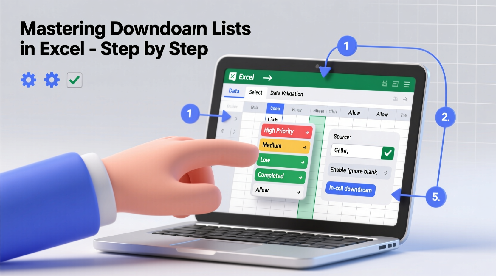
Start simple. Follow these steps to build a basic drop down list using Excel’s Data Validation feature:

1. Select the cell or range where you want the drop down (e.g., B2:B20).
2. Navigate to the Data tab on the ribbon.
3. Click Data Validation in the Data Tools group.
4. In the dialog box, set Allow to “List.”
5. In the Source field, enter comma-separated values (e.g., Yes,No,Maybe) or reference a range (e.g., =$E$2:$E$4).
6. Check “Ignore blank” and “In-cell dropdown” if desired.
7. Click OK.

The selected cells now display a small arrow. Clicking it reveals your predefined options. This method works well for static choices like status updates or priority levels.

Tip: Always define your source list in a separate worksheet or hidden column to keep your main sheet clean and avoid accidental edits.

Using Named Ranges for Cleaner Source References

Instead of hardcoding values or using direct cell references, use named ranges. They make formulas easier to read and maintain.

To create a named range:

• Select the list of items (e.g., E2:E5 containing “High,” “Medium,” “Low,” “Urgent”).
• Go to the Formulas tab.
• Click Define Name.
• Enter a meaningful name like “PriorityLevels” and click OK.

Now, in Data Validation, set the source as =PriorityLevels. If you later expand the list, update the named range, and all linked drop downs will reflect the change automatically.

Building Dynamic Drop Down Lists

Static lists are useful, but real-world scenarios often require adaptability. For example, selecting a country should only show relevant cities. This is where dynamic, dependent drop downs come in.

Creating a Dependent Drop Down

Suppose you have categories and subcategories:

Category	Subcategory
Electronics	Laptop
Electronics	Phone
Clothing	Shirt
Clothing	Pants

Steps to implement:

1. Create a table with categories and corresponding subcategories.
2. Name each subcategory column (e.g., “ElectronicsList” for laptops and phones).
3. In cell A2, create a primary drop down with Category options.
4. In B2, apply Data Validation with List type and source: =INDIRECT(A2).

The INDIRECT function converts the text in A2 into a range name. When “Electronics” is selected, Excel looks for a range named “Electronics” and populates the second drop down accordingly.

Tip: Ensure your named ranges exactly match the category names—including capitalization and spacing—to avoid #REF! errors.

Advanced Customization: Multi-Level Cascading Menus

For complex forms—like order entry systems—you may need three or more levels. Extend the dependent logic by nesting additional INDIRECT calls or using helper columns.

Example: Region → Country → City

• Region drop down in D2.
• Country in E2 uses =INDIRECT(D2).
• City in F2 uses =INDIRECT(E2), assuming countries are also named ranges.

This cascading structure prevents invalid combinations (e.g., selecting Tokyo under France) and guides users logically through selection paths.

Troubleshooting Common Issues

Even experienced users encounter glitches. Here are frequent problems and solutions:

Issue	Cause	Solution
Drop down shows #REF!	Named range deleted or misspelled	Recreate the named range; verify spelling
No options appear	Source range contains blank cells or typos	Remove blanks; ensure consistent formatting
Changes not updating	Named range not resized after adding items	Edit the named range to include new rows

Real-World Example: Project Task Tracker

A marketing team uses Excel to track campaign progress. Each task must be assigned a status: Not Started, In Progress, On Hold, Completed. To prevent inconsistent entries like “Done” or “Finished,” they implement a drop down in the Status column.

Beyond that, they add a second layer: when “On Hold” is selected, a comment automatically appears explaining why (via conditional formatting and cell notes). The team also creates a dynamic summary dashboard that counts tasks by status—only possible because entries are standardized.

Result: Reporting time drops from 30 minutes to under 5, and leadership gains confidence in the data.

Best Practices Checklist

Follow this checklist to ensure your drop down lists are effective and sustainable:

• ✅ Use separate sheets or columns for source lists.
• ✅ Apply named ranges instead of hardcoded values.
• ✅ Keep list items concise and mutually exclusive.
• ✅ Test dependent lists thoroughly after setup.
• ✅ Document list logic for future maintenance.
• ✅ Protect source ranges to prevent accidental deletion.
• ✅ Update named ranges when expanding lists.

Frequently Asked Questions

Can I allow users to add new items to a drop down list?

Not directly. Drop down lists based on data validation are fixed unless manually updated. However, you can design a companion form where new entries are added to the source list first, then refresh the named range. Alternatively, consider Power Query or VBA automation for advanced workflows.

Why does my drop down disappear when I filter data?

It doesn’t actually disappear—it’s still there, but filtered rows may hide the arrow. The functionality remains intact. Users can still click the cell and select from the list even if the dropdown icon isn’t visible due to screen rendering limitations in filtered views.

Can I have multiple selections in one drop down cell?

Standard Excel drop downs only allow one selection. For multiple entries, you’ll need workarounds such as concatenating inputs via VBA or using checkboxes linked to a hidden tracker. Alternatively, consider migrating to Microsoft Forms or SharePoint for richer input capabilities.

Conclusion: Take Control of Your Data

Mastering drop down lists transforms Excel from a passive calculator into an intelligent data collection tool. With proper setup, you reduce errors, speed up input, and lay the foundation for accurate reporting. These techniques scale from personal budgets to enterprise dashboards—any context where consistency matters.

🚀 Ready to upgrade your spreadsheets? Open an existing workbook today, identify one data entry point prone to inconsistency, and replace it with a smart drop down list. Small changes lead to big improvements in data quality.