Mastering How To Calculate Averages In Excel Tips And Tricks For Accurate Results

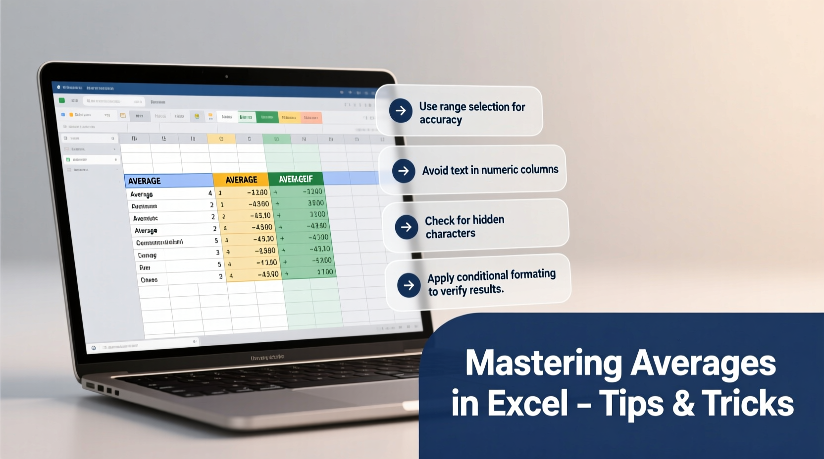
Accurate data analysis starts with reliable calculations—and one of the most fundamental operations in Excel is computing averages. Whether you're analyzing sales figures, student grades, or monthly expenses, understanding how to correctly calculate averages ensures your insights are both meaningful and trustworthy. While the AVERAGE function may seem straightforward, Excel offers a range of tools and nuances that can dramatically improve accuracy when used wisely.

Many users rely on basic formulas without realizing how outliers, blank cells, or conditional logic affect their results. Mastering average calculations means going beyond the basics—knowing when to use AVERAGEIF, how to handle errors gracefully, and ensuring your data reflects true central tendencies.

The Basics: How to Use the AVERAGE Function

The foundation of calculating averages in Excel is the AVERAGE function. It computes the arithmetic mean of a range of numbers by summing them and dividing by the count of numeric values.

Syntax:

=AVERAGE(number1, [number2], ...)

For example, if you have test scores in cells B2 through B10, the formula would be:

=AVERAGE(B2:B10)

This function automatically ignores text entries and empty cells but includes zero values in the calculation. That distinction is critical—if zeros represent missing data rather than actual performance, they can skew your average downward.

Tip: Always verify whether zero values are meaningful before using AVERAGE; otherwise, consider excluding them with conditional logic.

Handling Conditions: AVERAGEIF and AVERAGEIFS

Real-world datasets often require selective averaging based on criteria. For instance, you might want to find the average sales only for a specific region or calculate the mean score for students who passed an exam.

AVERAGEIF allows you to define a single condition:

=AVERAGEIF(range, criteria, [average_range])

Example: To average all sales greater than $500 in column C:

=AVERAGEIF(C2:C100, \">500\")

If multiple conditions apply, use AVERAGEIFS, which supports up to 127 criteria pairs:

=AVERAGEIFS(average_range, criteria_range1, criteria1, criteria_range2, criteria2, ...)

Suppose you want the average salary (column D) for employees in the \"Marketing\" department (column B) with more than two years of experience (column C):

=AVERAGEIFS(D2:D100, B2:B100, \"Marketing\", C2:C100, \">2\")

“Conditional averaging transforms raw data into targeted insights. Without it, decision-makers risk generalizing trends that don’t reflect specific segments.” — Dr. Lena Torres, Data Analyst & Business Intelligence Consultant

Dealing with Errors and Incomplete Data

Raw data is rarely perfect. Missing entries, typos, or error values like #DIV/0! and #N/A can disrupt average calculations. Excel provides several strategies to maintain integrity under these conditions.

Use AGGREGATE to ignore errors during averaging:

=AGGREGATE(1, 6, B2:B20)

Here, 1 represents AVERAGE, and 6 tells Excel to ignore error values.

Alternatively, wrap your formula with IFERROR to return a clean result instead of breaking the sheet:

=IFERROR(AVERAGE(B2:B20), \"Check data for errors\")

To exclude blank cells and zeros from consideration, combine AVERAGEIF with a logical test:

=AVERAGEIF(B2:B20, \"<>0\")

This excludes zero values, treating them as irrelevant rather than neutral contributors.

Step-by-Step Guide: Calculating a Weighted Average

Not all averages are created equal. When values carry different levels of importance—such as course grades weighted by credit hours—a simple average won't suffice.

Follow these steps to compute a weighted average:

1. List each value (e.g., grade) in one column and its corresponding weight (e.g., credits) in another.
2. Multiply each value by its weight (e.g., =B2*C2).
3. Sum the products using SUMPRODUCT.
4. Divide by the total weights using SUM.

Formula:

=SUMPRODUCT(values, weights) / SUM(weights)

Example: Grades in B2:B5, credits in C2:C5:

=SUMPRODUCT(B2:B5, C2:C5) / SUM(C2:C5)

Tip: Use named ranges (e.g., “Grades” and “Credits”) to make complex formulas easier to read and audit.

Common Pitfalls and Best Practices

Even experienced users fall into traps when calculating averages. Below is a summary of common mistakes and recommended actions.

Do’s	Don’ts
Verify data types—ensure numbers aren’t stored as text.	Assume Excel will always ignore non-numeric entries.
Use AVERAGEIF/S for filtering relevant subsets.	Apply AVERAGE to mixed-type columns without cleaning first.
Double-check cell references after inserting rows/columns.	Hardcode ranges instead of using dynamic tables or named ranges.
Consider median or trimmed means for skewed distributions.	Rely solely on average when outliers distort results.

Mini Case Study: Sales Performance Review

A regional manager at a retail chain wanted to assess quarterly performance across 15 stores. The initial report showed an average revenue per store of $48,200. However, upon closer inspection, one outlier—a flagship location generating $220,000—was inflating the overall figure.

By applying =TRIMMEAN(B2:B16, 0.2), which removes the top and bottom 10% of values before averaging, the adjusted average dropped to $39,600—providing a more realistic benchmark for typical store performance.

This insight led to revised targets and resource allocation, focusing support on underperforming locations rather than expecting uniform high output.

FAQ

Can I average cells based on font color or background color?

No, standard Excel functions don’t support formatting-based calculations. However, you can achieve this using VBA macros or by adding a helper column that flags colored cells via conditional logic.

Why does my AVERAGE function return a #DIV/0! error?

This occurs when there are no numeric values in the specified range. Check for text entries, hidden characters, or entirely blank ranges. Use IFERROR or validate input data to prevent disruption.

Is there a way to automatically update averages when new data is added?

Yes. Convert your data range into an Excel Table (Ctrl + T). Formulas referencing table columns will dynamically expand as new rows are added, keeping your averages current.

Conclusion: Turn Numbers Into Actionable Insights

Calculating averages in Excel is more than just typing a formula—it's about making informed decisions grounded in accurate data. From choosing the right function to handling edge cases and avoiding common errors, every step shapes the reliability of your conclusions.

Now that you understand how to leverage AVERAGE, AVERAGEIF, weighted methods, and error-resistant techniques, take a moment to review your existing spreadsheets. Are your averages telling the full story? Refine your approach, document your logic, and share your improved models with colleagues.

🚀 Ready to level up your Excel skills? Apply these tips today—recalculate one key average in your workbook with greater precision and see the difference firsthand.