Mastering How To Solve Linear Systems By Graphing A Step By Step Guide For Clear Understanding

Solving linear systems is a foundational skill in algebra, essential for modeling real-world relationships involving two variables. Among the various methods—substitution, elimination, and matrices—graphing offers a unique advantage: it provides a visual representation of solutions. When you can see where two lines intersect, abstract equations become tangible. This guide walks through the process of solving linear systems by graphing, breaking down each step with clarity, practical examples, and expert-backed insights.

Understanding Linear Systems and Their Graphical Meaning

A linear system consists of two or more linear equations that share the same variables. The most common form involves two equations with two variables (x and y). The solution to such a system is the set of values that satisfy all equations simultaneously. Graphically, each equation represents a straight line on the coordinate plane. The point where these lines intersect is the solution—the only (x, y) pair that works in both equations.

There are three possible outcomes when graphing a linear system:

• One solution: The lines intersect at a single point.
• No solution: The lines are parallel and never meet.
• Infinite solutions: The lines are identical (coinciding).

Understanding these outcomes helps interpret results not just mathematically, but contextually—especially in applications like break-even analysis or motion problems.

“Graphing transforms abstract equations into visual stories. It’s one of the best ways to build intuition about how variables interact.” — Dr. Alan Reyes, Mathematics Education Researcher

Step-by-Step Guide to Solving Linear Systems by Graphing

Follow this structured approach to confidently solve any linear system using graphing. Each step builds on the previous one, ensuring accuracy and comprehension.

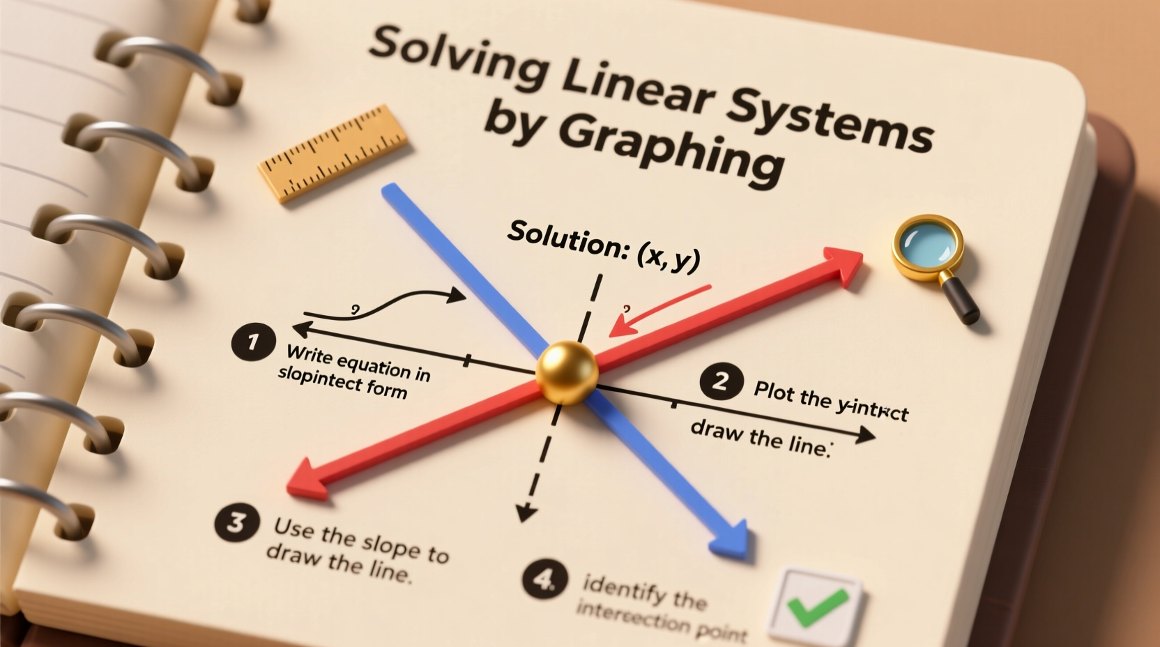
1. Write both equations in slope-intercept form (y = mx + b)
   Convert each equation so that y is isolated. This format reveals the slope (m) and y-intercept (b), making graphing straightforward.
2. Plot the y-intercepts of both lines
   Begin by marking the point where each line crosses the y-axis. For example, if an equation has b = 3, plot (0, 3).
3. Use the slope to find additional points
   From the y-intercept, apply the slope (rise over run) to locate another point. A slope of 2 means rising 2 units and running 1 unit to the right.
4. Draw both lines across the coordinate plane
   Connect the points for each equation with a straight line. Use a ruler if drawing manually, or extend the line logically.
5. Identify the point of intersection
   Locate where the two lines cross. This (x, y) coordinate is the solution.
6. Verify the solution algebraically
   Substitute the x and y values into both original equations to confirm they hold true.

Tip: Always double-check your equation conversion. A small error in rewriting y = 2x – 4 as y = 2x + 4 will shift the entire line and lead to an incorrect solution.

Real Example: Comparing Two Phone Plans

Consider a practical scenario: choosing between two phone plans based on cost and data usage.

Plan A: $20 monthly fee + $0.10 per GB of data
Plan B: $10 monthly fee + $0.15 per GB

The total cost equations are:

• Plan A: C = 0.10x + 20
• Plan B: C = 0.15x + 10

To find the break-even point (where both plans cost the same), graph both equations.

Convert to y = mx + b form (already done). Plot Plan A starting at (0, 20) with slope 0.10. Plan B starts at (0, 10) with slope 0.15. The steeper slope of Plan B means it increases faster. The lines intersect at (200, 40), meaning both plans cost $40 at 200 GB.

This graphical insight shows that under 200 GB, Plan B is cheaper; above that, Plan A wins. Visualizing this helps make informed decisions beyond mere calculations.

Common Mistakes and How to Avoid Them

Even simple graphs can lead to errors if care isn’t taken. Below is a summary of frequent pitfalls and how to prevent them.

Mistake	Why It Happens	How to Fix It
Incorrect slope application	Confusing rise/run direction or miscounting units	Double-check slope sign and use grid lines carefully
Faulty equation conversion	Algebra errors when isolating y	Re-solve step-by-step; verify with sample values
Poor scaling of axes	Choosing intervals that compress or stretch the graph	Select consistent, readable scales (e.g., 1, 2, 5, 10)
Assuming intersection without precision	Eye-balling instead of calculating exact coordinates	Use graph paper or digital tools; verify algebraically

Essential Tips for Accurate Graphing

Tip: Use different colors or line styles (dashed vs. solid) when sketching multiple lines. This makes it easier to distinguish them and track intersections.

• Always label your axes and include a scale.
• Extend lines far enough to ensure intersection (if expected) is visible.
• When graphing by hand, use graph paper for accuracy.
• If using digital tools (like Desmos or GeoGebra), verify manual work.
• Estimate fractional intersections carefully—zoom in or re-calculate if needed.

Checklist: Solving a Linear System by Graphing

Use this checklist before submitting your work or during practice sessions to ensure completeness and correctness.

1. ✅ Are both equations solved for y? (y = mx + b)
2. ✅ Have I correctly identified the slope and y-intercept for each?
3. ✅ Did I plot the y-intercepts accurately?
4. ✅ Did I use the slope to find at least one more point per line?
5. ✅ Are both lines drawn straight and extended across the grid?
6. ✅ Can I clearly identify the intersection point?
7. ✅ Have I verified the solution by plugging into both equations?

Frequently Asked Questions

What if the lines don’t intersect?

If two lines are parallel (same slope, different y-intercepts), they never intersect. This means the system has no solution and is called inconsistent. For example, y = 2x + 3 and y = 2x – 1 have no solution.

Can two equations graph as the same line?

Yes. If one equation is a multiple of the other (e.g., y = 2x + 4 and 2y = 4x + 8), they represent the same line. Every point on the line satisfies both equations, resulting in infinitely many solutions. This is a dependent system.

Is graphing always accurate?

Graphing provides a strong conceptual understanding, but it may lack precision—especially when solutions involve fractions or decimals. For exact answers, combine graphing with algebraic verification. In exams or real applications, always check your graphical result algebraically.

Conclusion: Turn Theory Into Practice

Mastering how to solve linear systems by graphing is more than a classroom exercise—it's a gateway to understanding relationships between variables in economics, physics, engineering, and everyday decision-making. With practice, the process becomes intuitive: convert, plot, draw, observe, verify. Each step reinforces both procedural fluency and conceptual depth.

Start with simple systems, use the checklist, and gradually tackle more complex ones. As confidence grows, so will your ability to interpret not just the \"how\" but the \"why\" behind the lines on the graph.

💬 Ready to test your skills? Grab a pencil and graph paper, pick two linear equations, and find their solution visually. Share your experience or ask questions in the comments—every graph tells a story worth discussing.