Proven Methods To Demonstrate Linearity In Maps A Step By Step Guide

Demonstrating linearity in maps—particularly in the context of linear transformations between vector spaces—is a foundational skill in linear algebra and functional analysis. Whether you're verifying a transformation in theoretical mathematics or applying it in machine learning, physics, or engineering, proving linearity ensures that operations preserve the structure of vector addition and scalar multiplication. This guide walks through the essential principles, verification steps, common pitfalls, and real-world applications to help you confidently establish linearity in any map.

Understanding Linearity: The Core Definition

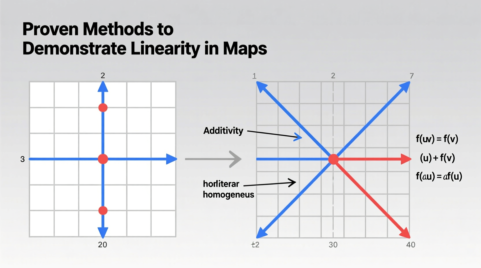
A map (or function) \\( T: V \\rightarrow W \\) between two vector spaces \\( V \\) and \\( W \\) over the same field (typically \\( \\mathbb{R} \\) or \\( \\mathbb{C} \\)) is said to be linear if it satisfies two properties for all vectors \\( \\mathbf{u}, \\mathbf{v} \\in V \\) and all scalars \\( c \\):

1. Additivity: \\( T(\\mathbf{u} + \\mathbf{v}) = T(\\mathbf{u}) + T(\\mathbf{v}) \\)
2. Homogeneity: \\( T(c\\mathbf{u}) = cT(\\mathbf{u}) \\)

These conditions ensure that the transformation respects the algebraic structure of the vector space. Together, they imply that \\( T \\) preserves linear combinations: \\( T(a\\mathbf{u} + b\\mathbf{v}) = aT(\\mathbf{u}) + bT(\\mathbf{v}) \\).

It's important to note that not all functions that \"look\" linear are actually linear. For example, affine maps like \\( f(x) = 2x + 3 \\) are not linear because they fail homogeneity unless the constant term is zero.

Tip: Always test both additivity and homogeneity independently. Skipping one condition can lead to incorrect conclusions.

Step-by-Step Guide to Proving Linearity

To rigorously prove that a given map is linear, follow this structured approach:

1. Identify the domain and codomain: Confirm that both \\( V \\) and \\( W \\) are vector spaces and that \\( T \\) is well-defined on \\( V \\).
2. State the general form of vectors: Let \\( \\mathbf{u}, \\mathbf{v} \\in V \\) be arbitrary elements, and let \\( c \\) be an arbitrary scalar.
3. Verify additivity: Compute \\( T(\\mathbf{u} + \\mathbf{v}) \\) and \\( T(\\mathbf{u}) + T(\\mathbf{v}) \\), then show they are equal using algebraic manipulation.
4. Verify homogeneity: Compute \\( T(c\\mathbf{u}) \\) and \\( cT(\\mathbf{u}) \\), then confirm equality.
5. Conclude linearity: If both properties hold for arbitrary inputs, the map is linear.

This method works whether you’re dealing with finite-dimensional spaces (like \\( \\mathbb{R}^n \\)), function spaces, or abstract vector spaces.

Example: Matrix Transformation

Let \\( T: \\mathbb{R}^2 \\rightarrow \\mathbb{R}^2 \\) be defined by \\( T(\\mathbf{x}) = A\\mathbf{x} \\), where \\( A = \\begin{bmatrix} 2 & 1 \\\\ 0 & 3 \\end{bmatrix} \\).

Take \\( \\mathbf{u} = \\begin{bmatrix} u_1 \\\\ u_2 \\end{bmatrix} \\), \\( \\mathbf{v} = \\begin{bmatrix} v_1 \\\\ v_2 \\end{bmatrix} \\), and scalar \\( c \\).

Additivity:
\\( T(\\mathbf{u} + \\mathbf{v}) = A(\\mathbf{u} + \\mathbf{v}) = A\\mathbf{u} + A\\mathbf{v} = T(\\mathbf{u}) + T(\\mathbf{v}) \\)

Homogeneity:
\\( T(c\\mathbf{u}) = A(c\\mathbf{u}) = c(A\\mathbf{u}) = cT(\\mathbf{u}) \\)

Since both conditions hold, \\( T \\) is linear.

Common Pitfalls and How to Avoid Them

Even experienced students and researchers can misidentify non-linear maps as linear due to superficial appearances. Here are frequent errors and how to prevent them:

Error Type	Description	How to Avoid
Assuming continuity implies linearity	Continuous functions aren't necessarily linear (e.g., \\( f(x) = x^2 \\)).	Always test the two axioms directly.
Overlooking constant terms	Affine maps like \\( T(x) = Ax + b \\) (with \\( b \ eq 0 \\)) fail homogeneity.	Check \\( T(0) \\); if \\( T(0) \ eq 0 \\), the map isn’t linear.
Misapplying operations in function spaces	In \\( C[0,1] \\), differentiation is linear, but squaring a function is not.	Test with specific functions like \\( f(x)=x \\), \\( g(x)=1 \\).
Confusing component-wise operations	Maps like \\( T(x,y) = (x^2, y) \\) appear structured but violate homogeneity.	Plug in a scalar multiple and verify algebraically.

Tip: Use the shortcut: if \\( T(\\mathbf{0}) \ eq \\mathbf{0} \\), the map cannot be linear. This quick check saves time.

Real-World Application: Linear Operators in Signal Processing

In digital signal processing, filters are often modeled as linear time-invariant (LTI) systems. Consider a discrete-time system defined by:

\\[ (T\\mathbf{x})[n] = \\sum_{k=-\\infty}^{\\infty} h[k]x[n-k] \\]

This is a convolution operator, commonly used in audio and image filtering. To prove linearity:

• Let \\( \\mathbf{x}_1, \\mathbf{x}_2 \\) be input signals, and \\( a, b \\) scalars.
• Compute \\( T(a\\mathbf{x}_1 + b\\mathbf{x}_2)[n] \\).
• Show it equals \\( aT(\\mathbf{x}_1)[n] + bT(\\mathbf{x}_2)[n] \\) using distributive property of summation.

This proof confirms that convolution is a linear operation, enabling superposition—a cornerstone of filter design and Fourier analysis.

“Linearity isn’t just a mathematical nicety—it’s what allows engineers to decompose complex signals into manageable parts.” — Dr. Lena Patel, Applied Mathematician at MIT

Checklist: Verifying Linearity in Practice

Use this checklist whenever analyzing a map for linearity:

• ✅ Confirm the domain and codomain are vector spaces.
• ✅ Check that \\( T(\\mathbf{0}) = \\mathbf{0} \\) (quick initial test).
• ✅ Write down expressions for \\( T(\\mathbf{u} + \\mathbf{v}) \\) and \\( T(\\mathbf{u}) + T(\\mathbf{v}) \\).
• ✅ Expand and simplify both sides; verify equality.
• ✅ Repeat for \\( T(c\\mathbf{u}) \\) and \\( cT(\\mathbf{u}) \\).
• ✅ Test with numerical examples if symbolic proof is unclear.
• ✅ Watch for non-linear operations: squares, absolute values, constants, or piecewise definitions without linearity.

Frequently Asked Questions

Can a map be partially linear?

No. Linearity is a strict binary condition. A map must satisfy both additivity and homogeneity for all inputs to be considered linear. If either fails—even at one point—the map is non-linear.

Is every matrix transformation linear?

Yes. Any function of the form \\( T(\\mathbf{x}) = A\\mathbf{x} \\), where \\( A \\) is a matrix, defines a linear transformation from \\( \\mathbb{R}^n \\) to \\( \\mathbb{R}^m \\). This follows directly from matrix algebra properties: \\( A(\\mathbf{u}+\\mathbf{v}) = A\\mathbf{u} + A\\mathbf{v} \\) and \\( A(c\\mathbf{u}) = c(A\\mathbf{u}) \\).

What about derivative and integral operators?

The derivative operator \\( D(f) = f' \\) on the space of differentiable functions is linear: \\( (af + bg)' = af' + bg' \\). Similarly, definite integration \\( I(f) = \\int_a^b f(x)\\,dx \\) is a linear functional. These are key examples in functional analysis and differential equations.

Conclusion: Building Confidence Through Rigorous Verification

Demonstrating linearity is more than a textbook exercise—it's a critical analytical tool across disciplines. From simplifying complex systems in engineering to validating models in data science, the ability to rigorously verify linearity strengthens your mathematical reasoning and problem-solving precision. By mastering the two core axioms, avoiding common traps, and applying structured verification, you equip yourself to handle increasingly sophisticated mappings with confidence.

💬 Ready to test your skills? Pick a transformation from your current work or studies and apply the step-by-step method today. Share your findings or questions in the discussion below.