Step By Step Guide To Building A Custom Amortization Schedule In Excel For Any Loan Type

An amortization schedule is a powerful financial tool that breaks down each payment on a loan into principal and interest over time. Whether you're managing a mortgage, auto loan, or personal installment loan, creating a custom schedule in Excel gives you full control and transparency. Unlike generic online calculators, a personalized spreadsheet allows you to adjust terms, rates, and extra payments with precision. This guide walks through the complete process of building a flexible, reusable amortization model from scratch.

Understanding Loan Amortization Basics

Amortization refers to the process of paying off a debt over time through regular installments. Each payment includes both interest (calculated on the remaining balance) and principal (the amount reducing the loan). Early payments are mostly interest; later ones are primarily principal. The standard formula for calculating the monthly payment on a fixed-rate loan is:

P = [r * PV] / [1 - (1 + r)^(-n)]

• P: Monthly payment
• r: Monthly interest rate (annual rate ÷ 12)
• PV: Present value or loan amount
• n: Total number of payments (loan term in years × 12)

This formula ensures consistent payments across the life of the loan. However, real-world loans may include variable rates, balloon payments, or irregular schedules—requiring customization beyond basic templates.

Tip: Always verify your interest rate format. If entering an annual rate of 5%, use 5% or 0.05 in Excel, not 5.

Step-by-Step Guide to Building Your Schedule

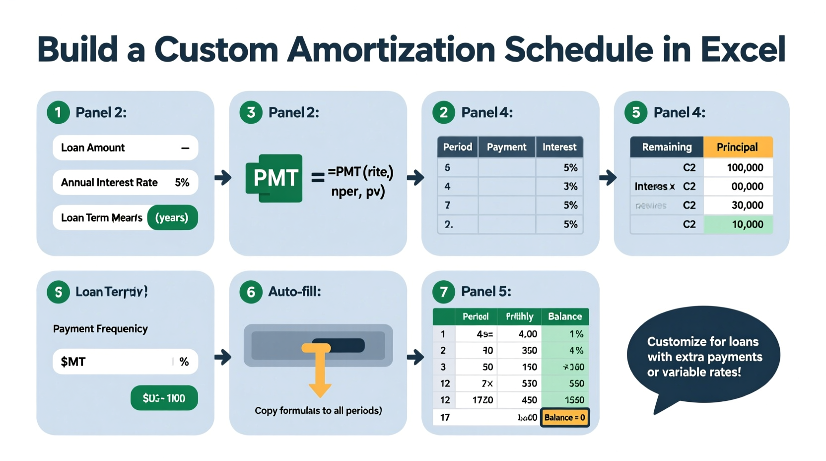
1. Set up input cells: Create labeled fields at the top of your worksheet for Loan Amount, Annual Interest Rate, Loan Term (Years), and Payments Per Year (usually 12).
2. Calculate derived values: Use formulas to compute the monthly rate, total number of payments, and monthly payment using the PMT function.
3. Create the amortization table: Begin a table with columns: Payment Number, Payment Date, Payment Amount, Principal, Interest, Extra Payment, and Remaining Balance.
4. Populate the first row: For Payment 1, calculate interest as =PreviousBalance * MonthlyRate, principal as =PaymentAmount - Interest, and new balance as =PreviousBalance - Principal - ExtraPayment.
5. Drag formulas down: Extend the table month by month until the balance reaches zero. Adjust end conditions if needed.

The key is ensuring that each row references the previous balance correctly. Circular references must be avoided unless intentional iterative calculations are enabled.

Incorporating Extra Payments

To model additional principal contributions—common in accelerated payoff strategies—add an \"Extra Payment\" column. This reduces the outstanding balance directly, shortening the loan term and cutting total interest paid.

Modify the ending balance formula to account for extras:

=PriorBalance - Principal - ExtraPayment

Use conditional logic to stop payments once the balance hits zero or goes negative:

=IF(RemainingBalance <= 0, \"\", PaymentAmount)

Advanced Customizations for Different Loan Types

Not all loans follow a standard fixed-payment structure. Here’s how to adapt your model:

• Variable-Rate Loans: Replace the fixed interest rate with a dynamic column where rates can change monthly or annually. Link to a separate assumptions sheet for clarity.
• Interest-Only Periods: During initial months, set principal to zero and only deduct interest. After the period ends, switch to full amortization.
• Biweekly Payments: Change the payment frequency to every two weeks (26 payments/year). Recalculate the periodic rate accordingly.
• Balloon Loans: Keep lower payments initially but retain a large final payment. Ensure the last row reflects the remaining balance instead of zeroing out.

Loan Type	Adjustment Needed	Key Formula Change
Adjustable Rate	Dynamic interest column	=INDEX(Rates, Month)
Interest-Only	Conditional principal	=IF(Month<=IO_Period, 0, Normal_Principal)
Biweekly	Frequency = 26	PMT(AnnualRate/26, Term*26, LoanAmount)
Balloon	Last payment ≠ regular amount	=RemainingBalance + Interest

“Building your own amortization schedule transforms passive borrowing into active financial management.” — James Reed, CFA and Financial Modeling Instructor

Checklist: Key Elements of a Robust Amortization Model

Checklist:

• ✅ Input section clearly separated from calculations
• ✅ Dynamic calculation of monthly payment via PMT()
• ✅ Accurate breakdown of principal and interest per period
• ✅ Support for extra payments without breaking the schedule
• ✅ Auto-stop when balance reaches zero
• ✅ Clear labeling and formatting for readability
• ✅ Optional: Summary dashboard showing total interest, payoff date, savings from extra payments

Real Example: Paying Off a $250,000 Mortgage Early

Consider a homeowner with a 30-year fixed mortgage at 6.5% APR on a $250,000 loan. Using the PMT function:

=PMT(6.5%/12, 360, 250000) returns a monthly payment of approximately $1,580.17.

Over 30 years, total interest would exceed $318,000. But by adding just $100 in extra principal each month, the loan pays off in about 25 years and 4 months—saving nearly $48,000 in interest.

In the amortization table, this adjustment appears as a dedicated column. By month 305, the balance drops below zero, signaling early payoff. The final payment adjusts automatically if you include logic like:

=IF(PriorBalance < PaymentAmount, PriorBalance + CurrentInterest, RegularPayment)

This flexibility makes Excel ideal for testing “what-if” scenarios before making financial decisions.

Frequently Asked Questions

Can I use this method for non-monthly loans?

Absolutely. Adjust the number of periods per year and recalculate the periodic interest rate. For quarterly loans, divide the annual rate by 4 and multiply the term in years by 4. Update the PMT function accordingly.

Why does my balance go negative at the end?

This happens when the final payment exceeds the remaining balance. Fix it by wrapping the payment amount in an IF statement: =IF(Balance < Payment, Balance + Interest, Payment). This ensures the last payment clears the balance without overpaying.

How do I handle loans with fees or upfront costs?

Include origination fees or closing costs in the initial loan balance if they’re financed. Alternatively, subtract them from net proceeds to reflect true borrowing cost. For APR calculations, incorporate these into effective rate analysis using Excel’s RATE() function.

Final Tips for Long-Term Use

Once built, save your amortization template as an Excel file (.xltx) for reuse. Add named ranges for inputs to make navigation easier. Protect formula cells while allowing input changes. Consider linking multiple scenarios (e.g., refinance vs. current loan) on separate tabs.

Track actual payments against projections to monitor progress. If your lender applies overpayments differently (e.g., to future payments instead of principal), adjust the model to match their policy—or request a recalculation.

Conclusion

Creating a custom amortization schedule in Excel empowers you to understand, control, and optimize your loan repayment strategy. From simple fixed-rate loans to complex structures with variable terms, the right model provides clarity and confidence. With accurate formulas, smart design, and scenario testing, you turn abstract debt into a visible, manageable path to financial freedom.

🚀 Ready to take control of your loan? Open Excel now, start building your schedule, and see exactly how fast you can become debt-free.